12 simple techniques for efficient work in Excel (9 photos + 5 hyphas)

To a human uninitiated, the Excel spreadsheet program seems huge, incomprehensible and therefore frightening.
In fact, this is a handy tool, and if you know the small tricks, you can greatly reduce the time to perform normal functions.
1. Quickly add new data to the chart:
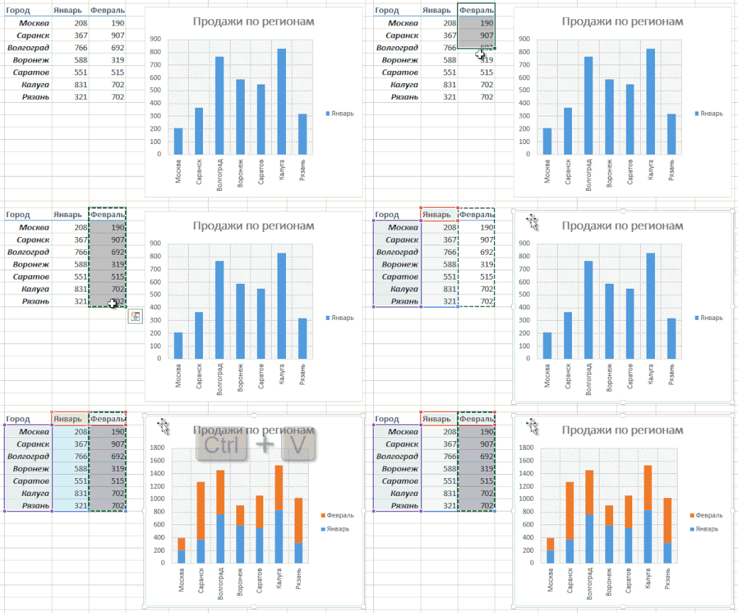
If for your chart you have already created new data to add, you can simply select the range with new information, copy it (Ctrl + C) and then paste it directly into the diagram (Ctrl + V).
2. Instant Fill (Flash Fill)
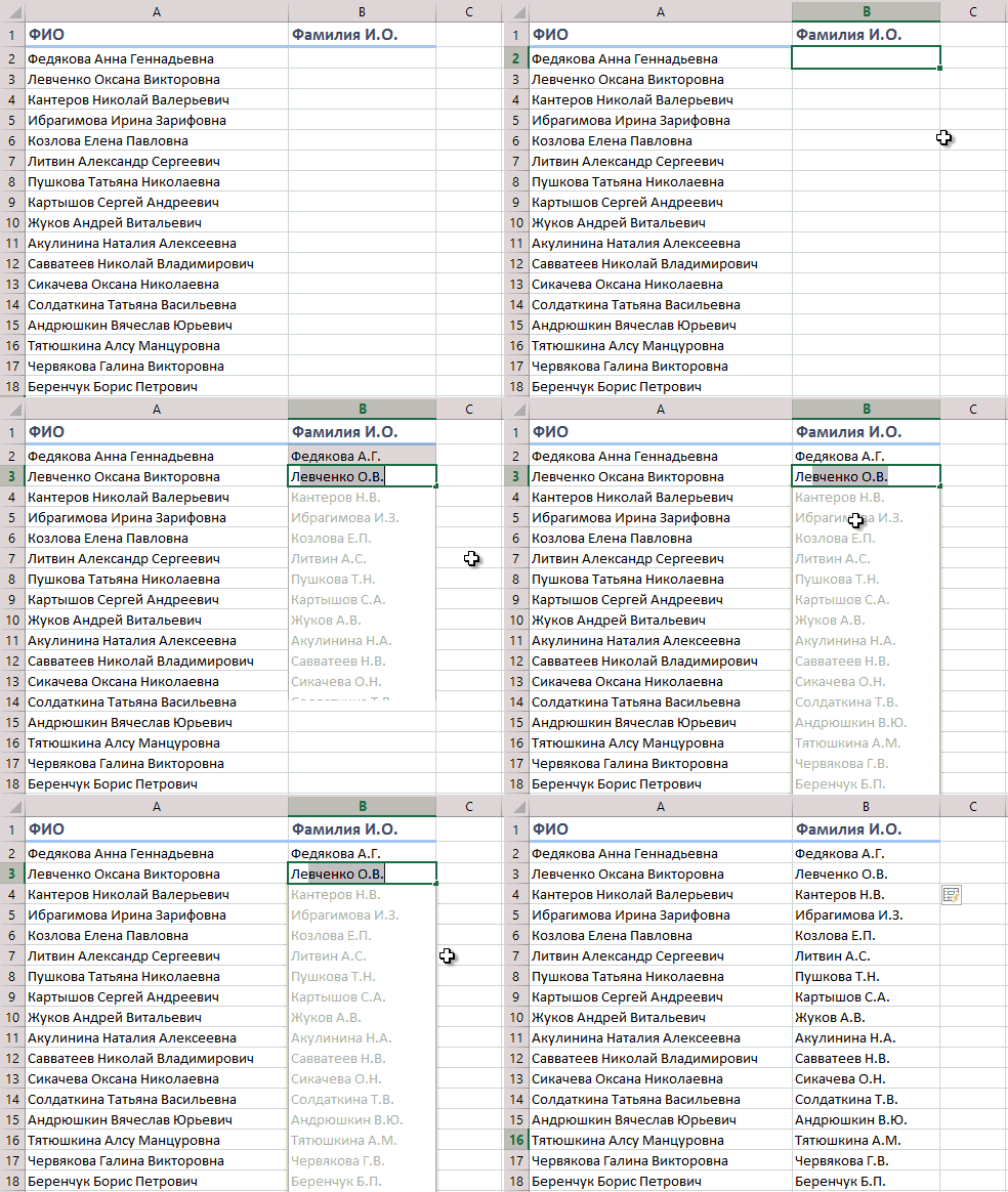
This function appeared only in the latest version of Excel 2013, but it is worth it to upgrade to the new version ahead of schedule. Suppose that you have a list of full names (Ivanov Ivan Ivanovich), which you need to turn into abbreviated ones (Ivanov II).
To perform such a conversion, you just need to start writing the desired text in the next column manually. On the second or third line, Excel will try to anticipate our actions and perform further processing automatically. You will only have to press the Enter key to confirm, and all the names will be converted instantly.
3. Copy without breaking the formats
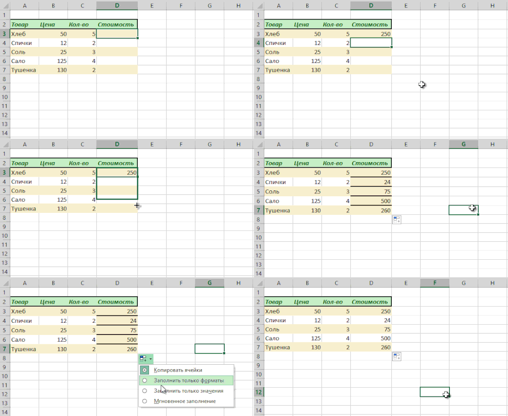
You probably know about the "magic" autocomplete token - a thin black cross in the lower right corner of the cell, pulling which you can copy the contents of the cell or the formula directly to several cells. However, there is one unpleasant nuance: such copying often violates the design of the table, because not only the formula is copied, but also the format of the cell. This can be avoided if immediately after dragging by a black cross click on the smart tag - a special icon that appears in the lower right corner of the copied area.
If you select the option "Fill Without Formatting", Microsoft Excel will copy your formula without format and will not spoil the design.
4. Displaying data from an Excel spreadsheet on a map
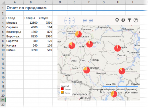
In the latest version of Excel 2013, you can quickly display on your interactive map your geographic data, for example, sales by city, etc. To do this, go to the "Office Store" on the "Insert" tab and install the Bing plug-in Maps.
This can be done and by direct link from the site, clicking the Add button. After adding the module, you can select it from the "My Apps" drop-down list on the "Insert" tab and place it on your worksheet. It remains to highlight your cells with data and click on the Show Locations button in the map module to see our data on it.
5. Quick jump to the desired sheet
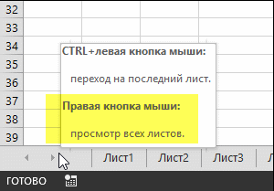
A table of contents appears, and you can switch to any desired sheet instantly.
You can also create a table of contents with hyperlinks on a separate sheet. This is a little more complicated, but often more convenient.
6. Convert rows to columns and back
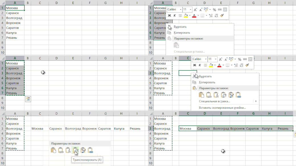
If you ever had to shift the cells from one row to the next, you'll appreciate the following trick:
Select the range.
Copy it (Ctrl + C) or, click on the right mouse button, select "Copy" (Copy).
Right-click on the cell where you want to insert the data, and select one of the special insertion options in the context menu - the "Transpose" icon.
In older versions of Excel, there is no such icon, but you can solve the problem with a special paste (Ctrl + Alt + V) and select the option "Transpose" (Transpose)
7. Drop-down list in the cell
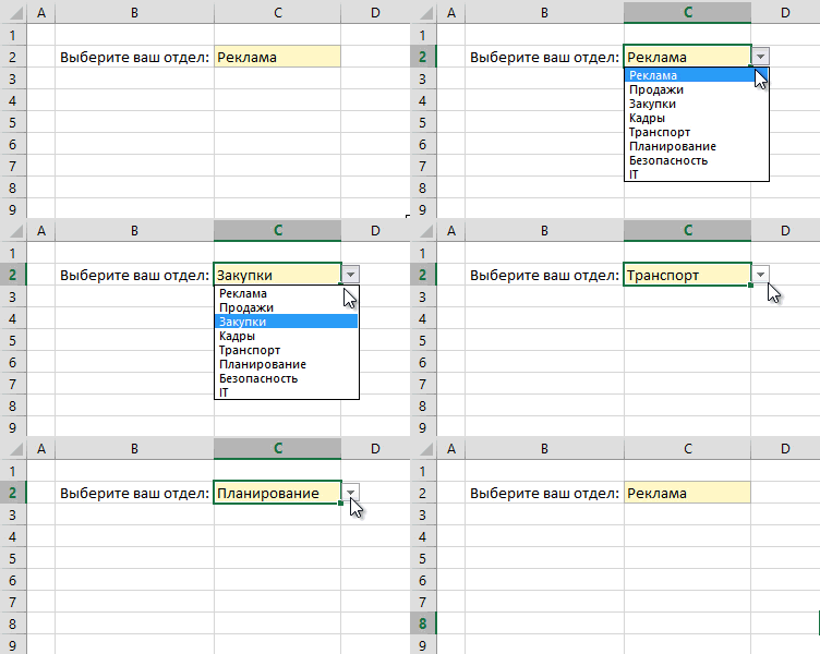
If a cell is supposed to enter strictly defined values from an allowed set (for example, only "yes" and "no" or only from the list of departments of the company, etc.), then it can be easily organized using the drop-down list:
Select the cell (or range of cells) in which there should be such a restriction.
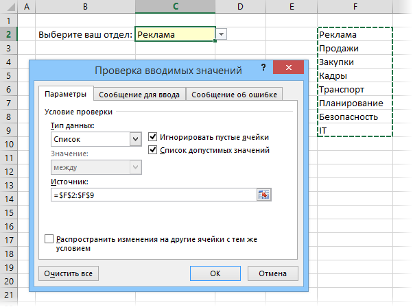
Click the "Validate Data" button on the "Data-Validation" tab.
In the "Type" drop-down list, select the "List" option.
In the "Source" field, specify the range containing the reference variants of the elements, which will subsequently drop out when you type.
8. "Smart" table
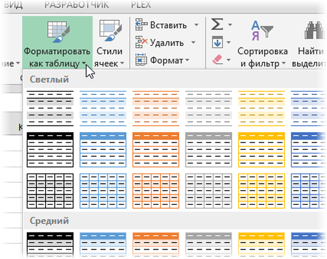
If you select a range with the data and click on the "Home" tab (Home - Format as Table), our list will be converted to a "smart" table, which (besides the fashion striped coloring) has many useful features:
Automatically stretch when you add new rows or columns to it.
The entered formulas automatically will be copied to the whole column.
The header of such a table is automatically fixed when scrolling, and the filter buttons for selecting and sorting are included in it.
On the appeared tab "Design" (Design) in such table it is possible to add a line of totals with automatic calculation.
9. Sparklines
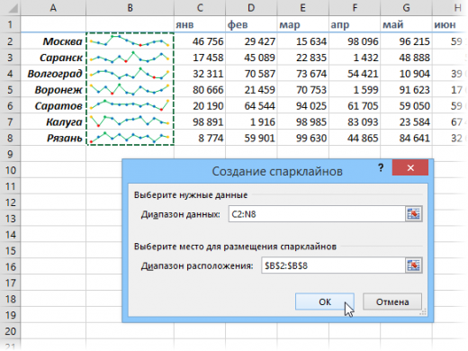
Sparklines are miniature diagrams drawn directly in the cells that clearly show the dynamics of our data. To create them, click the "Line" or "Columns" button in the "Sparklines" group on the "Insert" tab. In the window that opens, specify the range with the original numeric data and the cells where you want to display the sparklines.
After clicking on the "OK" button, Excel will create them in the specified cells. On the appeared tab "Design" (Design) it is possible to additionally adjust their color, type, include display of the minimum and maximum values, etc.
10. Restoring unsaved files

Friday. Evening. The long-awaited end of the shock work week. Anticipating the rest, you close the report with which you have been busy the last half of the day, and suddenly, for some reason, click "No" in the dialog "Save changes to the file?"
Empty office announces your heartrending cry, but it's too late - the last few hours of work have gone to hell and instead of having a pleasant evening with friends you will have to restore what you lost.
In fact, there is a strong chance to improve the situation. If you have Excel 2010, then click on "File" - "Recent" (File - Recent) and find the button in the lower right corner of the screen "Recover Unsaved Workbooks" (Recover Unsaved Workbooks). In Excel 2013, the path is slightly different: "File" - "Information" - "Version Control" - "Recover Unsaved Workbooks" (File - Properties - Recover Unsaved Workbooks). A special folder from the depths of Microsoft Office opens, where for this case, temporary copies of all created or modified, but unsaved books are saved.
11. Comparison of the two ranges for differences and coincidences
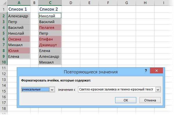
Quite often when working in Excel, it becomes necessary to compare two lists and quickly find the elements that match or differ in them. The fastest and most visible way to do this is:
Select both columns to compare (hold down the Ctrl key).
Select on the Home tab - Conditional Formatting - Cell Selection Rules - Home-Conditional formatting - Highlight Cell Rules - Duplicate Values.
Select "Unique" from the drop-down list.
12. Selection (fitting) the results of the calculation to the desired values
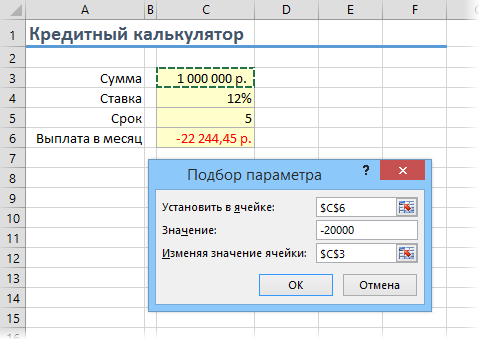
Have you ever picked up input values in your Excel calculation to get the output you want? At such times, you feel like a martial artilleryman, right? Just a couple of dozen iterations "not long - flight", and here it is, the long-awaited "hit"!
Microsoft Excel can do this for you, and faster and more accurately. To do this, click on the "Insert" tab, the "Analysis" button that if "" and select the "Insert - What If Analysis - Goal Seek" command. In the window that appears, specify the cell where you want to select the desired value, the desired result and the input cell, which should change. After clicking on "OK" Excel will execute up to 100 "shots" to find the required result with an accuracy of 0.001.


Comments
Commenting on, remember that the content and tone of your message can hurt the feelings of real people, show respect and tolerance to your interlocutors even if you do not share their opinion, your behavior in the conditions of freedom of expression and anonymity provided by the Internet, changes Not only virtual, but also the real world. All comments are hidden from the index, spam is controlled.